Autoencoders compress data to a code, then reconstruct it. But the learned codes have no structure; nearby codes don't correspond to similar data. VAEs add probabilistic structure, creating smooth latent spaces where you can sample new data and interpolate between examples.
Why Sutskever Included This
VAEs bridge probabilistic reasoning and deep learning. They provide a principled way to learn latent representations that support generation. The ideas (ELBO optimization, reparameterization, latent variable models) recur throughout modern generative AI.
The Autoencoder Problem
Standard autoencoders learn encoder E(x) → z and decoder D(z) → x'. They minimize reconstruction error ||x - x'||². The learned z codes are deterministic.
Problem: the latent space has gaps. If z₁ encodes a cat and z₂ encodes a dog, there's no guarantee the midpoint (z₁ + z₂)/2 encodes anything sensible. You can't sample new codes and expect meaningful outputs.
Probabilistic Encoding
VAEs make encoding probabilistic. The encoder outputs parameters of a distribution: mean μ and variance σ², not a single code. The latent z is sampled from this distribution.
Encoder: x → (μ, σ²)
Sample: z ~ N(μ, σ²)
Decoder: z → x'
Training encourages the encoded distributions to match a prior (typically standard normal). This regularizes the latent space, filling gaps and enabling sampling.
The ELBO
VAEs maximize the Evidence Lower Bound:
ELBO = E[log p(x|z)] - KL(q(z|x) || p(z))
First term: reconstruction quality. Second term: regularization toward the prior.
The KL divergence penalizes encodings that deviate from the standard normal prior. This creates overlap between different inputs' latent distributions, filling the space.
The Reparameterization Trick
Sampling z ~ N(μ, σ²) breaks gradient flow. You can't backpropagate through a random sample. The reparameterization trick fixes this:
z = μ + σ × ε, where ε ~ N(0, 1)
Now the randomness (ε) is external. Gradients flow through μ and σ normally. This simple change made VAE training practical.
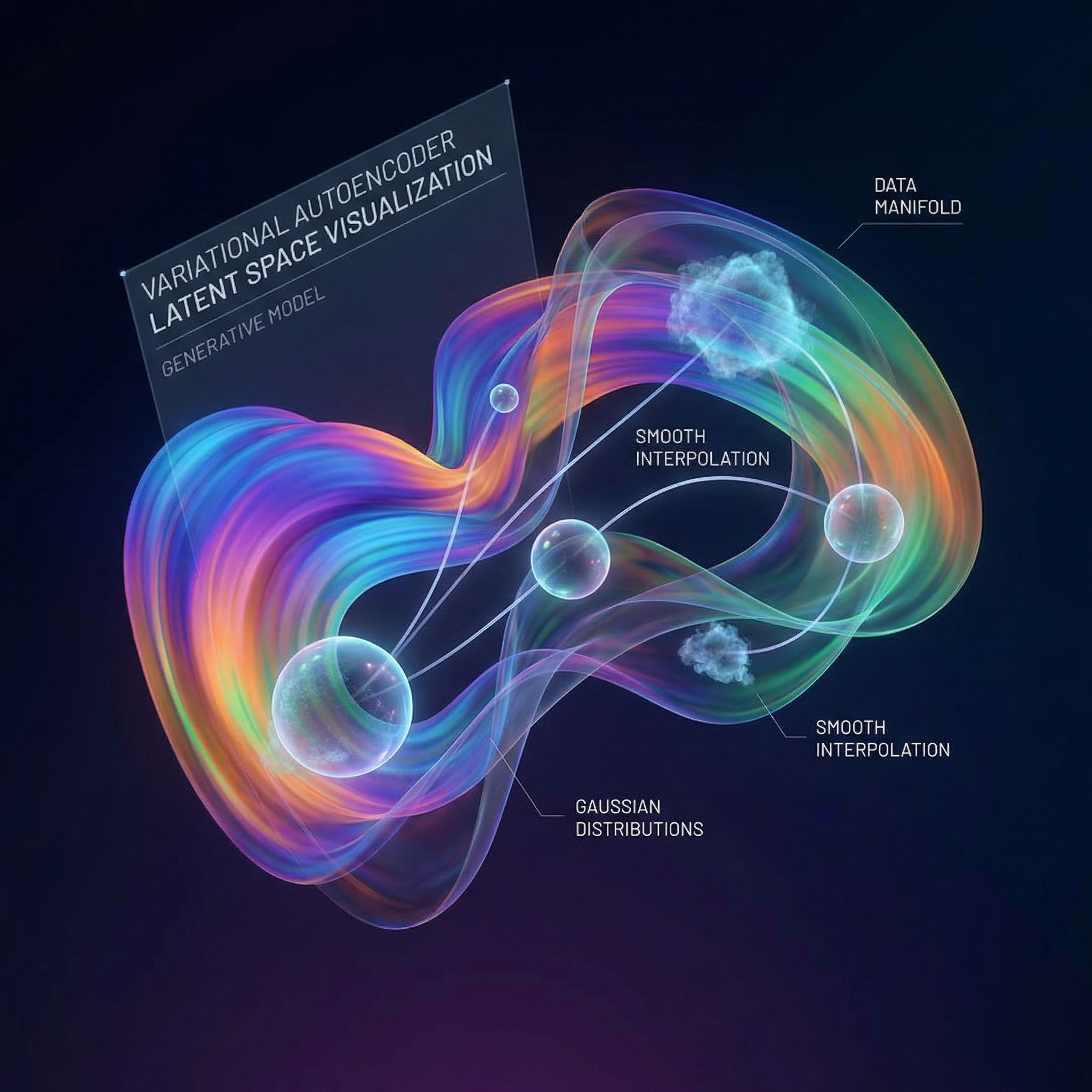
Latent Space Properties
Continuity: Nearby points decode to similar outputs. Moving smoothly through latent space morphs between data examples.
Completeness: Any point sampled from the prior decodes to plausible data. No dead regions in the latent space.
Interpolation: The path between two encoded points shows meaningful intermediate forms. Blend a 3 and an 8; see digits that morph between them.
Limitations
VAE reconstructions tend toward blurriness. The Gaussian decoder assumption encourages averaging over possibilities rather than committing to sharp details.
GANs produce sharper images but lack the structured latent space. Diffusion models offer both quality and structure. VAEs were a stepping stone toward these more capable approaches.
Applications
Representation learning: VAE latent codes capture meaningful factors of variation. Use them as features for downstream tasks.
Data augmentation: Sample new training examples from the latent space.
Anomaly detection: Unusual inputs have high reconstruction error. VAEs naturally flag out-of-distribution data.
Further Reading
More in This Series
Part of a series on Ilya Sutskever's recommended 30 papers.